
Characterizing the Dynamics of Covid-19 Based on Data
Abstract
The objective of this paper is to apply datadriven discovery of dynamics modeling to obtain a system of differential equations that allows us to describe the transmission dynamics of Covid-19, based on the number of confirmed cases and deaths reported daily. This methodology was applied in four different countries: Brazil, Colombia, Venezuela, and the United States. The main advantage is that only one differential equation is needed to characterize the dynamic of Covid-19 without any mathematical assumption.
Article Information
- Received
- Accepted
- Published
Academic Editor: Qianqian Song, Wake Forest School of Medicine, Wake Forest Baptist Comprehensive Cancer Center, Medical Center Boulevard, Winston-Salem, NC 27157.
Checked for plagiarism: Yes
Review by: Single-blind
Copyright © 2021 Raúl Isea
 This is an open-access article distributed under the terms of the Creative Commons Attribution License, which permits unrestricted use, distribution, and reproduction in any medium, provided the original author and source are credited.
Corresponding author: Correspondence: Raúl Isea, Fundación Instituto de Estudios Avanzados, Hoyo de la Puerta, Baruta, Venezuela —
Competing Interests
The authors have declared that no competing interests exist.
Funding
No specific funding statement was provided by the authors.
Data Availability
No data-availability statement was provided by the authors.
Acknowledgements
I’d like to acknowledgment to Rafael Mayo-Garcia and Jesus Isea for your comments in this manuscript.
Citation:
Introduction
There is a great effort to explain the transmission dynamics of Covid-19 with mathematical models after it was declared a pandemic in March 2020 1. In fact, a search in Google Scholar (to cite an example) using the keywords: "Mathematics + Covid-19", obtained 17,900 different results from 2020 as those of November 2021. All of it indicates the great diversity of results obtained in this important field of work.
Most of these papers are dedicated to describe the outbreak in some places of the world. For example, Isea described the dynamics on Venezuela 2, Tang et al on Brazil 3, and so on. For that reason, it is necessary to develop a methodology that allows describing the epidemic by Covid-19 based on the data, and principally with only a mathematical model.
In the last decade, computational methodologies have been developed for obtaining the non-linear differential equations that rule a dynamical system. One of the techniques to do so is called datadriven discovery of dynamics modeling 4, 5, 6, 7, which is based on Sparse Identification of Nonlinear Dynamics (SINDy). This computational implementation is usually done in Python 8 or Mathematical 9.
In fact, the SINDy methodology applied to Covid-19 has already been reported in the scientific literature see for example 10, but unlike those publications, we obtained a polynomial differential equation based on confirmed cases and deaths reported daily as described in the next section.
Methodology
The data driven discovery of equations is a computational methodology where applied techniques of Data Science and Machine Learningare used, and also Artificial Intelligence as shown by Bruton et al7. This methodology is displayed in Figure 1, where only solutions of polynomial functions are considered.
As can be seen in Figure 1, a matrix whose columns are the time dependent input data are built, i.e., the number of confirmed cases (I) and deaths (D) reported daily. The next step was to build a library of coefficients of nonlinear functions based on polynomial function indicated as in the figure, where the degree of a polynomial is represented by U. For example, U=2, it means will be [1, I,D,I2,D2,ID] (1 in these expressions represents a constant value).
Figure 1. Schematic illustration of the methodology to calculate the differential equations (T means transpose). 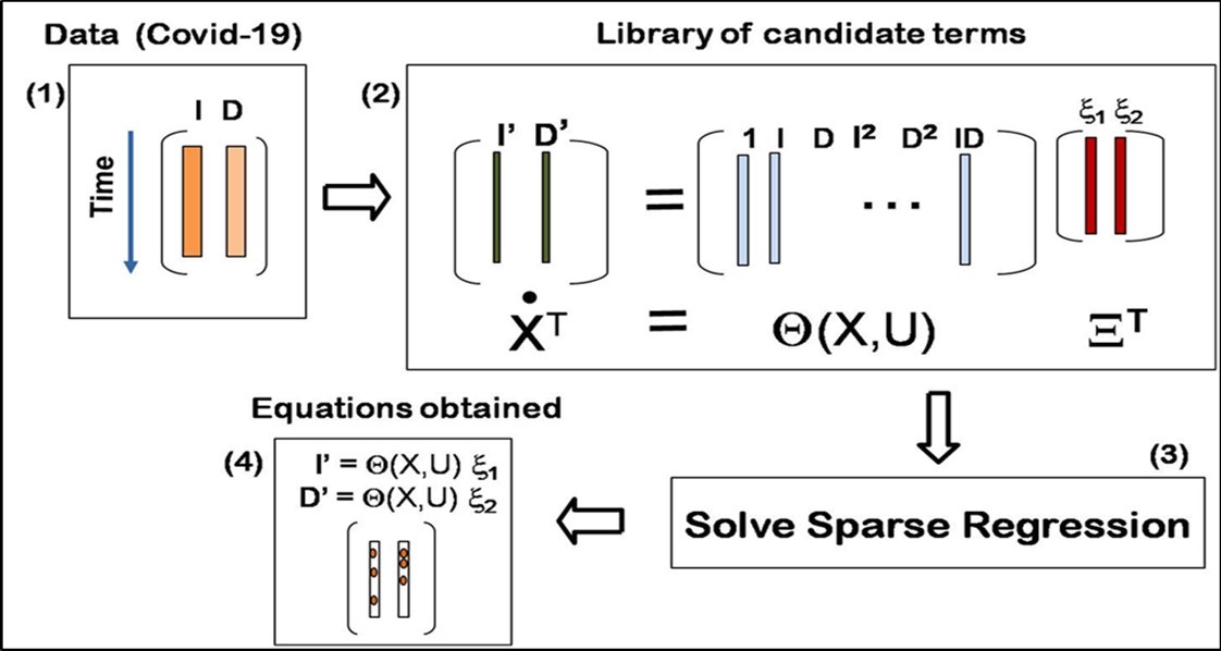
Download figure
The dynamics will be described by the following equation (the point in X represents the derivative respect to the time), and the sparse coefficients vector will be equal to [x1, x2,], which correspond to the values of [I, D], respectively (accordingly to Bruton’s methodology)7.
The third step is an optimization process where the parameters are calculated by Least Absolute Shrinkage and Selection Operator (abbreviated as LASSO) 14. Remember that LASSO regression is also known as L1-norm regression. In future papers other methods will be implemented such as Scaled Sequential Threshold Least Squares (S2TLS) algorithm 15 to compare results. This step is really the most import of them all. In fact, the degree (U) in the library coefficients is obtained automatically by the program according to the minimization of the error in the optimization step.
Finally, the last step is to obtain the differential equation. For the case in which U=2, this would be

where ai and bi (i from 1 to 6) are the constant coefficients to be calculated for each of the countries.
Results
The data was obtained from the Johns Hopkins University portal, available at coronavirus.jhu.edu. Four countries were selected: Brazil, Colombia, Venezuela, and the United States, and in each country the numberof contagions (I) and deaths (D) is obtained, from March 27, 2020 until June 14, 2021 (a total of 445 records) were retrieved.
The next step was to normalize the data according to standard deviation, and the results are shown in figure 2, i.e., this normalization consisted of subtracting by the mean value and divided by the standard deviation, where the data was represented by symbols in blue color, and the results obtained in dashedblack line. It is interesting to see the result in Brazil by the dispersion of the data.
Figure 2. Daily cases records versus time (t) on the United States, Brazil, Colombia, and Venezuela represented with a blue point, and with dash line shows the results obtained in the normalization of the data. 
Download figure
The next step was to calculate the parameters with the normalization data according to with the methodology described in Figure 1, where the library of coefficients of nonlinear functions is based on a polynomial function. The coefficients obtained in each country are shown in Table 1. The degree of differential equations obtained in all countries wasthree (U=3, error less than 0.001). In addition, it is interesting to note how different are the parameters obtained in this table, because each result depends on country response measures to Covid-19.
Table 1. Coefficients obtained in the differential equations system (1) on Brazil (BRA), United States (USA), Venezuela (VEN), and Colombia (COL), divided into two sections corresponding to dI/dt and dD/dt, respectively.

|

|
 D D |
 I I |

|

|

|

|

|

|

|
| BRA | 0,15 | 0,34 | 0,04 | 15,8 | 14,0 | -29,8 | 63,3 | -55,1 | -24,0 | 15,8 |
| USA | 0,10 | 0,24 | 3,00 | -1,43 | 4,88 | -2,01 | -3,03 | 0,22 | ||
| VEN | -3,66 | 7,97 | -7,46 | 13,3 | -8,73 | 17,3 | -26,6 | 9,90 | ||
| COL | 0,02 | 10,0 | -8,13 | -58,1 | -66,5 | 123,5 | -657,9 | 664,2 | -224,2 | 218,2 |

|

|
 D D |
 I I |

|

|

|

|

|

|

|
| BRA | 0,34 | 1,64 | -2,52 | 14,3 | 13,3 | -26,7 | 10,7 | -5,52 | -5,29 | |
| USA | 0,10 | 0,20 | -0,77 | -2,55 | -2,99 | 6,54 | -0,46 | 0,002 | 0,18 | |
| VEN | -4,10 | 7,17 | -1,82 | 18,5 | -18,5 | 15,8 | -24,0 | 8,59 | ||
| COL | 0,04 | 14,8 | -13,3 | -58,4 | -72,3 | 130,0 | 644,9 | -641,5 | -217,3 | 214, |
Finally, figure 3 depicts the result obtained in (A) the United States of America and (B) Venezuela according to the results obtained in Table 1 (the results are shown with a red line). The results show that this methodology is not capable to make accurate predictions when there is a lot of difference in the number of cases (see for example the US case), while the prediction for Venezuela better reproduces the observed cases.
Figure 3. Results obtained in (A) the United States, and (B) Venezuela. Daily cases record are shown in blue point, the result obtained with the SINDy methodology in dashed black line (represented as SG), and the values obtained according to the coefficients indicated in Table 1in red. 
Download figure
Conclusion
This paper proposes a system of differential equations of the polynomial type that allows characterizing the transmission dynamics of Covid-19 in any country since the beginning of the pandemic. The main advantage of this methodology is that it is possible to derive only one differential equation to explain the dynamics of contagion by SARS-CoV-2. It only remains to indicate that it is necessary to develop numerical calculations to be able to generalize these conclusions.
Dedication
This paper is dedicated to the memory to Gloria Teresa Villegas who died on 21th October 2021. Her husband, Raimundo Villegas, also died on October 21. Thank you for your friendship.
References
- 2.Isea R. (2020) Simulando la dinamica del Covid-19 desde una perspectivematematica. Revista Observador del. , Conocimiento 5, 13-19.
- 3.Tang Y, Serdan TDA, Alecrim A L, Souza D R, Nacano BRM et al. (2021) . , Scientific Report 11, 16400.
- 4.Godal P, Benner P. (2021) Discovery of nonlinear dynamical system using a Runge-Kutta inspired dictionary-based sparse regression approch. ArXiv:. 2105-04869.
- 5.Subber W, Pandita P, Ghosh S, Khan G, Wang L et al. (2020) Data-based discovery of governing equations. 2012-06036.
- 6.Pantazis Y, Tsamardinos I. (2019) A unified approach for sparse dynamical system inferece from temporal measurements. , Bioinformatics 35(18), 3387-3396.
- 7.Brunton S L, Proctor J L, Kutz J N. (2016) Discovering governing equationsfrom data by sparse identification of nonlinear dynamics systems. , Proc. Nath. Acad. Scie 113, 3932-3937.
- 8.B De Silva, Champion K, Quade M, Loiseau J C, Kutz J N et al. (2020) PySINDY: A python package for the sparse identification of nonlinear dynamics from data. arXiv:. 2004-08424.
- 9.Kaiser E, Kutz J N, Brunton S L. (2017) Sparse identification of nonlinear dynamics for model predictive control in the low-data limit. arXiv:. 1711-05501.
- 10.Larson K, Bowman C, Chen Z, Hadjidoukas P, Papadimitriou C et al. (2020) Data-driven prediction and origin identification of epidemics in population networks. 1710-078802.
- 11.Pal D, Ghosh D, Santra P K, Mahapatra G S. (2020) Mathematical analysis of a Covid-19 epidemic model by using Data Driven epidemiological parameters of disease in India. medRxiv: https://doi.org/10.1101/2020.04.25.20079
- 12.Kuhl E. (2020) Data-driven modeling of Covid-19-Lessons learned. , Extreme Mechanics Letters 40, 100921.
Cited by (2)
This article has been cited by 2 scholarly works according to:
Citing Articles:
Journal of Model Based Research (2023) OpenAlex Crossref Semantic Scholar